Parameter estimation and distribution selection by ExtDist

Introduction

Parameter estimation and distribution selections are common tasks in statistical analysis. In the context of variables acceptance sampling (see Wu and Govindaraju 2014 etc.), when the underlying distribution model of the quality characteristic is determined, the estimated quality of a product batch measured by the proportion nonconforming, is computed through the estimated parameter(s) of the underlying distribution based on a sample. Conversely, if a collection of candidate distributions are considered to be eligible, then selection of a distribution that best describes the data becomes necessary.

The package is devoted to provide a consistent and unified framework for these tasks.

library(ExtDist)

Parameter Estimation

Suppose we have a set of data, which has been randomly generated from a Weibull distributed population,

set.seed(1234)
head(X <- rWeibull(50, shape = 2, scale = 3))

[1] 4.423512 2.066157 2.111723 2.062377 1.160961 2.003052

It is possible to write code to obtain parameters via a maximum likelihood estimation procedure for the data. However, it is more convenient to use a single function to achieve this task.

est.par <- eWeibull(X)

The \(e-\) prefix we introduced in is a logical extension to the \(d-\), \(p-\), \(q-\), \(r-\) prefixes of the distribution-related functions in R base package. Moreover, the output of \(e-\) functions is defined as a S3 class object.

class(est.par)

[1] "eDist"

The estimated parameters stored in the “eDist” object can be easily plugged into other \(d-\), \(p-\), \(q-\), \(r-\) functions in to get the density, percentile, quantile and random variates for a distribution with estimated parameters.

dWeibull(seq(0,2,0.4), params = est.par)
pWeibull(seq(0,2,0.4), params = est.par)
qWeibull(seq(0,1,0.2), params = est.par)
rWeibull(10, params = est.par)

To remain compatible with current convention, these functions also accept the parameters as individual arguments, so the following code variations are also permissible.

dWeibull(seq(0,2,0.4), shape = est.par$shape, scale = est.par$scale)
pWeibull(seq(0,2,0.4), shape = est.par$shape, scale = est.par$scale)
qWeibull(seq(0,1,0.2), shape = est.par$shape, scale = est.par$scale)
rWeibull(10, shape = est.par$shape, scale = est.par$scale)

Distribution selection

As a S3 class object, several S3 methods have been developed in to extract the distribution selection criteria and other relevant information.

logLik(est.par) # log likelihood

[1] -79.99344

AIC(est.par) # Akaike information criterion
AICc(est.par) # corrected Akaike information criterion

[1] 164.2422

BIC(est.par) # Bayes' Information Criterion.

[1] 167.8109

MDL(est.par) # minimum description length

[1] 83.03809

vcov(est.par) # variance-covariance matrix of the parameters of the fitted distribution

           shape      scale
shape 0.06609441 0.01566200
scale 0.01566200 0.03801099

Based on these criteria, for any sample, the best fitting distribution can be obtained from a list of candidate distributions. For example:

Ozone <- airquality$Ozone
Ozone <- Ozone[!is.na(Ozone)] # Removing the NA's from Ozone data
summary(Ozone)

   Min. 1st Qu.  Median    Mean 3rd Qu.    Max. 
   1.00   18.00   31.50   42.13   63.25  168.00

best <- bestDist(Ozone, candDist=c("Gamma", "Weibull", "Normal", "Exp"), criterion = "logLik");best

[1] "Weibull"
attr(,"best.dist.par")

Parameters for the Weibull distribution. 
(found using the  numerical.MLE method.)

 Parameter  Type  Estimate       S.E.
     shape shape  1.340187 0.09541768
     scale scale 46.081330 3.37566679


attr(,"criterion.value")
    Gamma   Weibull    Normal       Exp 
     -Inf -542.6103 -569.6492 -549.9263

When more than one set of results are of interest for a list of candidate distribution fits, a summary table can be output by using the function DistSelCriteria.

DistSelCriteria(Ozone, candDist = c("Gamma", "Weibull", "Normal", "Exp"),
                         criteria = c("logLik","AIC","AICc", "BIC"))

       Gamma Weibull   Normal    Exp      
logLik -Inf  -542.6103 -569.6492 -549.9263
AIC    Inf   1089.221  1143.298  1101.853 
AICc   Inf   1089.327  1143.404  1101.888 
BIC    Inf   1094.728  1148.805  1104.606

Multiple distributions can also be compared visually using the compareDist function.

compareDist(Ozone, attributes(best)$best.dist.par, eNormal(Ozone))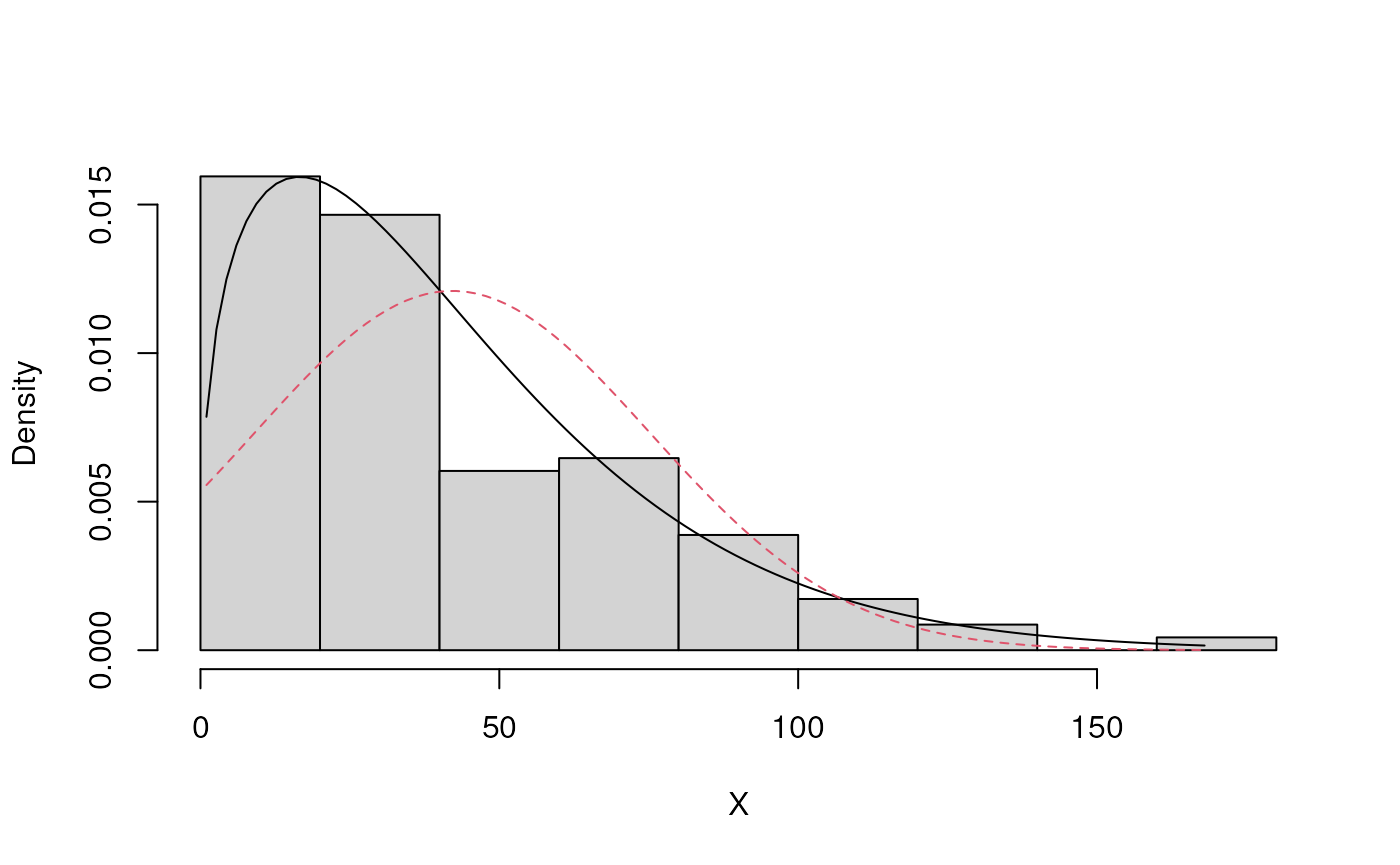

If the best fit distribution has been determined plot.eDist can provide the corresponding histogram with fitted density curve, Q-Q and P-P plot for this distribution.

plot(attributes(best)$best.dist.par)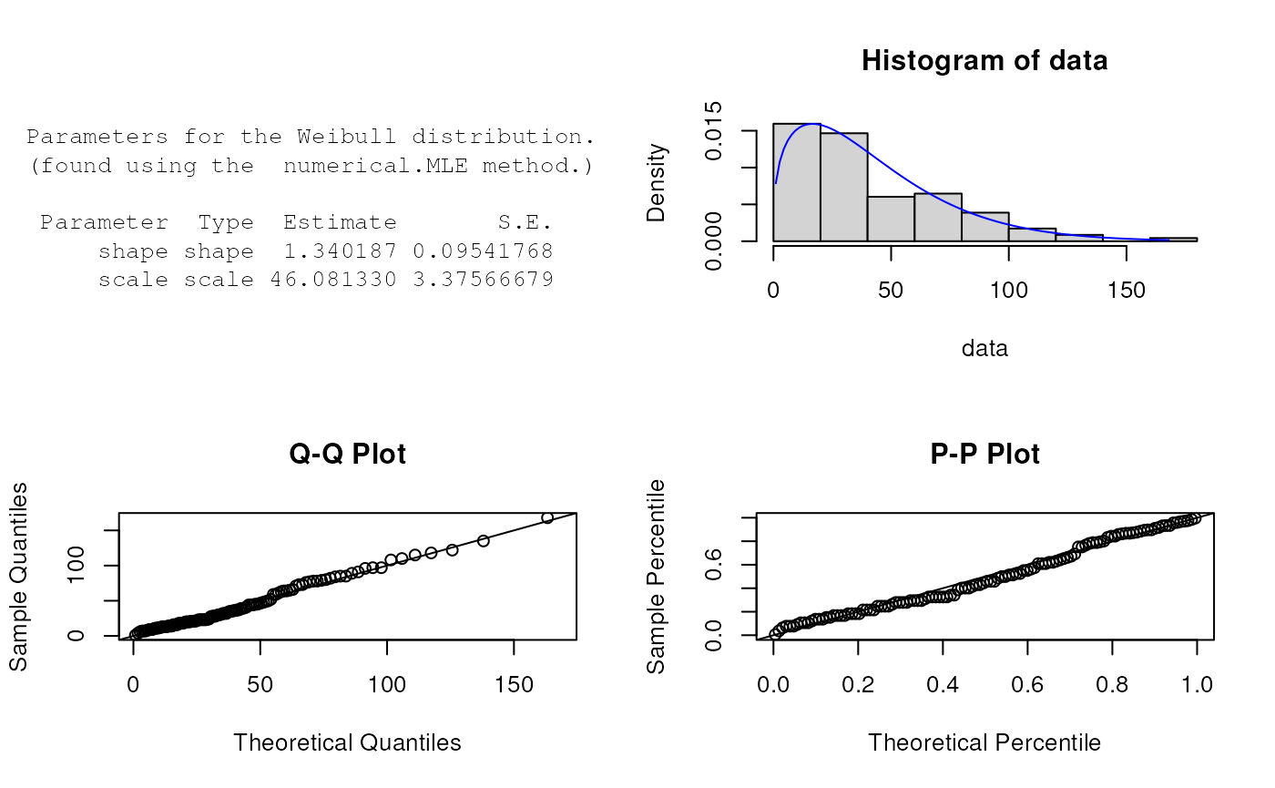

Weighted sample

Another notable feature of the package is that it can deal with weighted samples. Weighted samples appear in many contexts, e.g.: in non-parametric and semi-parametric deconvolution (see e.g. Hazelton and Turlach 2010 etc.) the deconvoluted distribution can be represented as a pair \((Y,w)\) where \(w\) is a vector of weights with same length as \(Y\). In size-biased (unequal probability) sampling, the true population is more appropriately described by the weighted (with reciprocal of the inclusion probability as weights) observations rather than the observations themselves. In Bayesian inference, the posterior distribution can be regarded as a weighted version of the prior distribution. Weighted distributions can also play an interesting role in stochastic population dynamics.

In , the parameter estimation was conducted by maximum weighted likelihood estimation, with the estimate \(\hat{\boldsymbol{\theta}}\) of \(\boldsymbol{\theta}\) being defined by \[\begin{align}\label{eq:1} \hat{\boldsymbol{\theta}}^{w}=\arg\max_{\boldsymbol{\theta}}\sum_{i=1}^n w_i\ln f(Y_i;\boldsymbol{\theta}), \end{align}\] where \(f\) is the density function of the ditstribution to be fitted.

For example, for a weighted sample with

Y <- c(0.1703, 0.4307, 0.6085, 0.0503, 0.4625, 0.479, 0.2695, 0.2744, 0.2713, 0.2177, 
       0.2865, 0.2009, 0.2359, 0.3877, 0.5799, 0.3537, 0.2805, 0.2144, 0.2261, 0.4016)
w <- c(0.85, 1.11, 0.88, 1.34, 1.01, 0.96, 0.86, 1.34, 0.87, 1.34, 0.84, 0.84, 0.83, 1.09, 
       0.95, 0.77, 0.96, 1.24, 0.78, 1.12)

the parameter estimation and distribution selection for weighted samples can be achieved by including the extra argument \(w\):

eBeta(Y,w)


Parameters for the Beta distribution. 
(found using the  MOM method.)

 Parameter  Type Estimate
    shape1 shape 3.016450
    shape2 shape 6.561803

bestDist(Y, w, candDist = c("Beta_ab","Laplace","Normal"), criterion = "AIC")

[1] "Normal"
attr(,"best.dist.par")

Parameters for the Normal distribution. 
(found using the  unbiased.MLE method.)

 Parameter     Type  Estimate       S.E.
      mean location 0.3149269 0.03157766
        sd    scale 0.1412196 0.02290885


attr(,"criterion.value")
  Beta_ab   Laplace    Normal 
-14.76974 -17.67491 -18.10897

DistSelCriteria(Y, w, candDist = c("Beta_ab","Laplace","Normal"),
                         criteria = c("logLik","AIC","AICc", "BIC"))

       Beta_ab   Laplace   Normal   
logLik 11.38487  10.83745  11.05448 
AIC    -14.76974 -17.67491 -18.10897
AICc   -12.10308 -16.96903 -17.40309
BIC    -10.78682 -15.68344 -16.11751

References

Hazelton, Martin L., and Berwin A. Turlach. 2010. “Semiparametric Density Deconvolution.” Scandinavian Journal of Statistics 37 (1): 91–108.

Wu, Haizhen, and Kondaswamy Govindaraju. 2014. “Computer-aided variables sampling inspection plans for compositional proportions and measurement error adjustment.” Computers & Industrial Engineering 72 (June): 239–46.

Haizhen Wu, A. Jonathan R. Godfrey and Sarah Pirikahu

2023-08-23

Introduction

Parameter Estimation

Distribution selection

Weighted sample

References