Density, distribution, and quantile, random number generation,
and parameter estimation functions for the logistic distribution with parameters location and scale.
Parameter estimation can be based on a weighted or unweighted i.i.d. sample and can be carried out numerically.
dLogistic(
  x,
  location = 0,
  scale = 1,
  params = list(location = 0, scale = 1),
  ...
)

pLogistic(
  q,
  location = 0,
  scale = 1,
  params = list(location = 0, scale = 1),
  ...
)

qLogistic(
  p,
  location = 0,
  scale = 1,
  params = list(location = 0, scale = 1),
  ...
)

rLogistic(
  n,
  location = 0,
  scale = 1,
  params = list(location = 0, scale = 1),
  ...
)

eLogistic(X, w, method = "numerical.MLE", ...)

lLogistic(
  X,
  w,
  location = 0,
  scale = 1,
  params = list(location = 0, scale = 1),
  logL = TRUE,
  ...
)
Arguments
- x, q
A vector of quantiles.
- location
Location parameter.
- scale
Scale parameter.
- params
A list that includes all named parameters.
- ...
Additional parameters.
- p
A vector of probabilities.
- n
Number of observations.
- X
Sample observations.
- w
An optional vector of sample weights.
- method
Parameter estimation method.
- logL
logical; if TRUE, lLogistic gives the log-likelihood, otherwise the likelihood is given.
Value
dLogistic gives the density, pLogistic the distribution function, qLogistic the quantile function, rLogistic generates random deviates, and eLogistic estimates the parameters. lLogistic provides the log-likelihood function.
Details
If location or scale are omitted, they assume the default values of 0 or 1
respectively.
The dLogistic(), pLogistic(), qLogistic(),and rLogistic() functions serve as wrappers of the
standard dlogis, plogis, qlogis, and
rlogis functions in the stats package. They allow for the parameters to be declared not only as
individual numerical values, but also as a list so parameter estimation can be carried out.
The logistic distribution with location = \(\alpha\) and scale = \(\beta\) is most simply
defined in terms of its cumulative distribution function (Johnson et.al pp.115-116)
$$F(x) = 1- [1 + exp((x-\alpha)/\beta)]^{-1}.$$
The corresponding probability density function is given by
$$f(x) = 1/\beta [exp(x-\alpha/\beta][1 + exp(x-\alpha/\beta)]^{-2}$$
Parameter estimation is only implemented numerically.
The score function and Fishers information are as given by Shi (1995) (See also Kotz & Nadarajah (2000)).
References
Johnson, N. L., Kotz, S. and Balakrishnan, N. (1995) Continuous Univariate Distributions, volume 2,
chapter 23. Wiley, New York.
Shi, D. (1995) Fisher information for a multivariate extreme value distribution, Biometrika, vol 82, pp.644-649.
Kotz, S. and Nadarajah (2000) Extreme Value Distributions Theory and Applications, chapter 3, Imperial Collage Press,
Singapore.
See also
ExtDist for other standard distributions.
Examples
# Parameter estimation for a distribution with known shape parameters
X <- rLogistic(n=500, location=1.5, scale=0.5)
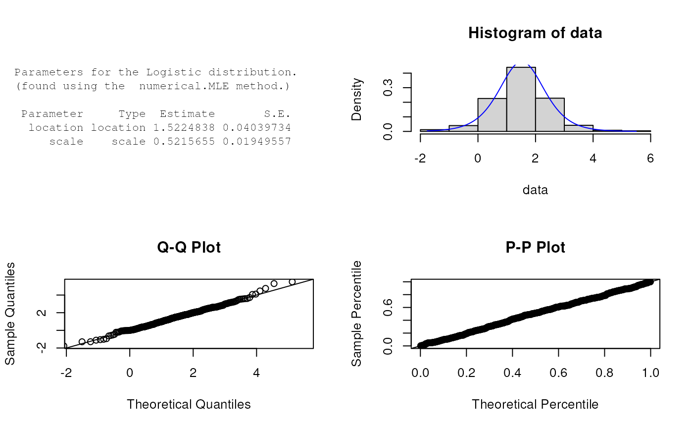
est.par <- eLogistic(X); est.par
#>
#> Parameters for the Logistic distribution.
#> (found using the numerical.MLE method.)
#>
#> Parameter Type Estimate S.E.
#> location location 1.5553977 0.03768637
#> scale scale 0.4880874 0.01830572
#>
#>
plot(est.par)
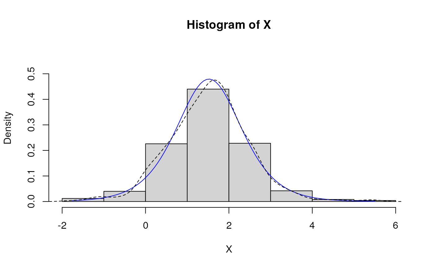
 # Fitted density curve and histogram
den.x <- seq(min(X),max(X),length=100)
den.y <- dLogistic(den.x,location=est.par$location,scale=est.par$scale)
hist(X, breaks=10, probability=TRUE, ylim = c(0,1.2*max(den.y)))
lines(den.x, den.y, col="blue")
lines(density(X), lty=2)
# Fitted density curve and histogram
den.x <- seq(min(X),max(X),length=100)
den.y <- dLogistic(den.x,location=est.par$location,scale=est.par$scale)
hist(X, breaks=10, probability=TRUE, ylim = c(0,1.2*max(den.y)))
lines(den.x, den.y, col="blue")
lines(density(X), lty=2)
 # Extracting location or scale parameters
est.par[attributes(est.par)$par.type=="location"]
#> $location
#> [1] 1.555398
#>
est.par[attributes(est.par)$par.type=="scale"]
#> $scale
#> [1] 0.4880874
#>
# log-likelihood function
lLogistic(X,param = est.par)
#> [1] -643.7141
# Evaluation of the precision of the parameter estimates by the Hessian matrix
H <- attributes(est.par)$nll.hessian
fisher_info <- solve(H)
var <- sqrt(diag(fisher_info));var
#> location scale
#> 0.03768637 0.01830572
# Example of parameter estimation for a distribution with
# unknown parameters currently been sought after.
# Extracting location or scale parameters
est.par[attributes(est.par)$par.type=="location"]
#> $location
#> [1] 1.555398
#>
est.par[attributes(est.par)$par.type=="scale"]
#> $scale
#> [1] 0.4880874
#>
# log-likelihood function
lLogistic(X,param = est.par)
#> [1] -643.7141
# Evaluation of the precision of the parameter estimates by the Hessian matrix
H <- attributes(est.par)$nll.hessian
fisher_info <- solve(H)
var <- sqrt(diag(fisher_info));var
#> location scale
#> 0.03768637 0.01830572
# Example of parameter estimation for a distribution with
# unknown parameters currently been sought after.