The Johnson SB distribution.

Density, distribution, quantile, random number generation, and parameter estimation functions for the Johnson SB (bounded support) distribution. Parameter estimation can be based on a weighted or unweighted i.i.d. sample and can be performed numerically.

dJohnsonSB(
  x,
  gamma = -0.5,
  delta = 2,
  xi = -0.5,
  lambda = 2,
  params = list(gamma = -0.5, delta = 2, xi = -0.5, lambda = 2),
  ...
)

dJohnsonSB_ab(
  x,
  gamma = -0.5,
  delta = 2,
  a = -0.5,
  b = 1.5,
  params = list(gamma = -0.5, delta = 2, a = -0.5, b = 1.5),
  ...
)

pJohnsonSB(
  q,
  gamma = -0.5,
  delta = 2,
  xi = -0.5,
  lambda = 2,
  params = list(gamma = -0.5, delta = 2, xi = -0.5, lambda = 2),
  ...
)

qJohnsonSB(
  p,
  gamma = -0.5,
  delta = 2,
  xi = -0.5,
  lambda = 2,
  params = list(gamma = -0.5, delta = 2, xi = -0.5, lambda = 2),
  ...
)

rJohnsonSB(
  n,
  gamma = -0.5,
  delta = 2,
  xi = -0.5,
  lambda = 2,
  params = list(gamma = -0.5, delta = 2, xi = -0.5, lambda = 2),
  ...
)

eJohnsonSB(X, w, method = "numerical.MLE", ...)

lJohnsonSB(
  X,
  w,
  gamma = -0.5,
  delta = 2,
  xi = -0.5,
  lambda = 2,
  params = list(gamma = -0.5, delta = 2, xi = -0.5, lambda = 2),
  logL = TRUE,
  ...
)

Arguments

x, q: A vector of quantiles.
gamma, delta: Shape parameters.
xi, lambda, a, b: Location-scale parameters.
params: A list that includes all named parameters.
...: Additional parameters.
p: A vector of probabilities.
n: Number of observations.
X: Sample observations.
w: An optional vector of sample weights.
method: Parameter estimation method.
logL: logical, it is assumed that the log-likelihood is desired. Set to FALSE if the likelihood is wanted.

Value

dJohnsonSB gives the density, pJohnsonSB the distribution function, qJohnsonSB gives quantile function, rJohnsonSB generates random deviates, and eJohnsonSB estimate the parameters. lJohnsonSB provides the log-likelihood function. The dJohnsonSB_ab provides an alternative parameterisation of the JohnsonSB distribution.

Details

The Johnson system of distributions consists of families of distributions that, through specified transformations, can be reduced to the standard normal random variable. It provides a very flexible system for describing statistical distributions and is defined by $$z = \gamma + \delta f(Y)$$ with $Y = (X-xi)/lambda$. The Johnson SB distribution arises when $f(Y) = ln[Y/(1-Y)]$, where $0 < Y < 1$. This is the bounded Johnson family since the range of Y is $(0,1)$, Karian & Dudewicz (2011).

The dJohnsonSB(), pJohnsonSB(), qJohnsonSB(),and rJohnsonSB() functions serve as wrappers of the dJohnson, pJohnson, qJohnson, and rJohnson functions in the SuppDists package. They allow for the parameters to be declared not only as individual numerical values, but also as a list so parameter estimation can be carried out.

The JohnsonSB distribution has probability density function $$p_X(x) = \frac{\delta lambda}{\sqrt{2\pi}(x-xi)(1- x + xi)}exp[-0.5(\gamma + \delta ln((x-xi)/(1-x+xi)))^2].$$

References

Johnson, N. L., Kotz, S. and Balakrishnan, N. (1994) Continuous Univariate Distributions, volume 1, chapter 12, Wiley, New York.

Kotz, S. and van Dorp, J. R. (2004). Beyond Beta: Other Continuous Families of Distributions with Bounded Support and Applications. Appendix B. World Scientific: Singapore.

Z. A. Karian and E. J. Dudewicz (2011) Handbook of Fitting Statistical Distributions with R, Chapman & Hall.

Author

Haizhen Wu and A. Jonathan R. Godfrey.
Updates and bug fixes by Sarah Pirikahu.

Examples

# Parameter estimation for a distribution with known shape parameters
X <- rJohnsonSB(n=500, gamma=-0.5, delta=2, xi=-0.5, lambda=2)
est.par <- eJohnsonSB(X); est.par
#> 
#> Parameters for the JohnsonSB distribution. 
#> (found using the  numerical.MLE method.)
#> 
#>  Parameter     Type   Estimate       S.E.
#>      gamma    shape -0.3194679 0.17707240
#>      delta    shape  1.5821162 0.20959773
#>         xi location -0.2316520 0.17210297
#>     lambda    scale  1.6166668 0.08039103
#> 
#> 
plot(est.par)


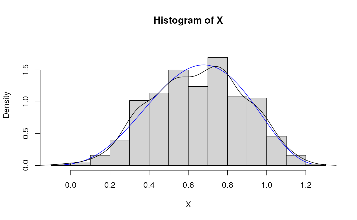
#  Fitted density curve and histogram
den.x <- seq(min(X),max(X),length=100)
den.y <- dJohnsonSB(den.x,params = est.par)
hist(X, breaks=10, probability=TRUE, ylim = c(0,1.2*max(den.y)))
lines(den.x, den.y, col="blue")
lines(density(X))


# Extracting location, scale and shape parameters
est.par[attributes(est.par)$par.type=="location"]
#> $xi
#> [1] -0.231652
#> 
est.par[attributes(est.par)$par.type=="scale"]
#> $lambda
#> [1] 1.616667
#> 
est.par[attributes(est.par)$par.type=="shape"]
#> $gamma
#> [1] -0.3194679
#> 
#> $delta
#> [1] 1.582116
#> 

# Parameter Estimation for a distribution with unknown shape parameters
# Example from Karian, Z.A and Dudewicz, E.J. (2011) p.647.
# Original source of brain scan data Dudewich, E.J et.al (1989).
# Parameter estimates as given by Karian & Dudewicz using moments are:
# gamma =-0.2081, delta=0.9167, xi = 95.1280 and lambda = 21.4607 with log-likelihood = -67.03579
brain <- c(108.7, 107.0, 110.3, 110.0, 113.6, 99.2, 109.8, 104.5, 108.1, 107.2, 112.0, 115.5, 108.4,
           107.4, 113.4, 101.2, 98.4, 100.9, 100.0, 107.1, 108.7, 102.5, 103.3)
est.par <- eJohnsonSB(brain); est.par
#> 
#> Parameters for the JohnsonSB distribution. 
#> (found using the  numerical.MLE method.)
#> 
#>  Parameter     Type   Estimate
#>      gamma    shape  0.0491309
#>      delta    shape  0.6547437
#>         xi location 97.9208050
#>     lambda    scale 18.0843462
#> 
#> 

# Estimates calculated by eJohnsonSB differ from those given by Karian & Dudewicz (2011).
# However, eJohnsonSB's parameter estimates appear to be an improvement, due to a larger
# log-likelihood of -66.35496 (as given by lJohnsonSB below).

# log-likelihood function
lJohnsonSB(brain, param = est.par)
#> [1] -66.35496